Labels

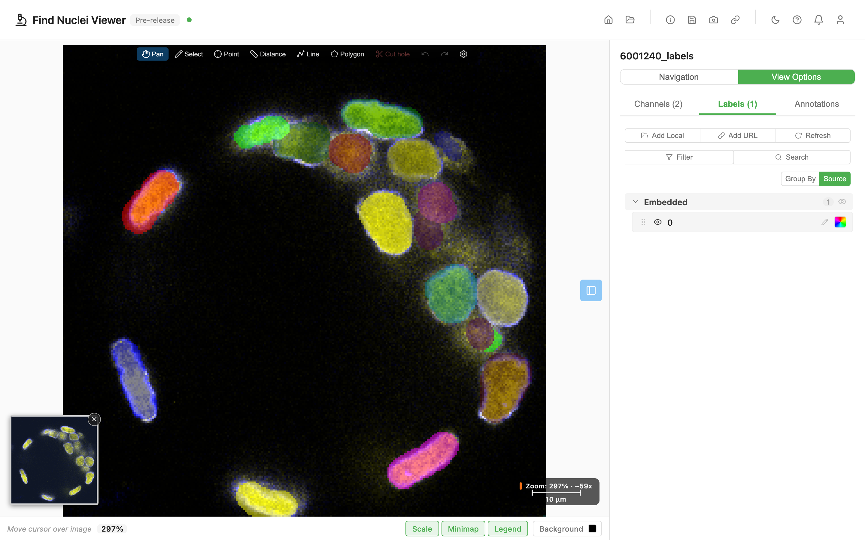
A label is a segmentation mask: one integer per pixel, where each integer is an object ID. Labels live alongside your image and render as a coloured overlay so you can see what was detected by your segmentation tool (CellProfiler, Cellpose, StarDist, InstanSeg, and anything else that writes OME-Zarr or bare Zarr masks).

This guide covers the foundational workflow: load labels, control how they look, organise them, attach metadata. For per-object coloring by measurement CSVs (heatmap, category, phenotypes), see the Analytics & Phenotyping guide.

Loading labels

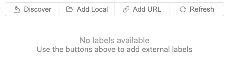
The buttons at the top of the Labels tab:

Button	What it does
Add Local	Pick a folder on your disk that contains a Zarr label array. Chrome / Edge only.
Add URL	Paste a URL pointing at a Zarr label array. Works in any browser.
Discover	Scan an HCS plate's fields for labels. Only appears on plates, and only runs when you click it. See below.
Refresh	Re-scan the current image's OME-Zarr for embedded labels. Useful if a segmentation job has just written a new label and you don't want to reload the whole image.

Embedded labels

Labels written inside your OME-Zarr (under the /labels/ group, per the OME-NGFF spec) are discovered automatically on image load. No clicking required. They appear in the Embedded group in the list.

Plates: press Discover

On an HCS plate, labels are not discovered automatically. You get a Discover button instead, and nothing is scanned until you press it.

This is deliberate. The scan asks every well whether it has a labels/ group, so a 384-well plate is 384 requests before a single pixel is drawn. Ten run in parallel, and only field 0 of each well is checked, but the count still scales with the plate. Against a local disk that is merely slow. Against S3 it is 384 billed requests every time anyone opens the plate, whether or not they wanted labels at all. So the scan is something you ask for, not something that happens to you.

Because it visits every well, the result knows which wells actually carry each label, rather than assuming the whole plate matches the first one.

Press Discover once and the labels stay attached for the session. If a segmentation job writes new masks while you have the plate open, press it again.

Local folders (Add Local)

Click Add Local, pick any folder containing a Zarr label. The folder stays on your disk. The viewer reads it directly via the File System Access API. Use this when you've run a segmentation tool that wrote a Zarr mask next to (but not inside) your image.

Remote URLs (Add URL)

Click Add URL and paste the URL of a Zarr label array. Works from any storage that serves HTTP range requests and the right CORS headers: S3, Cloudflare R2, GCS, Azure Blob, an on-premise nginx, a data server running locally. See the Data Server guide for hosting your own.

External labels (not embedded in the image's OME-Zarr) show an EXT badge in the list so you can tell them apart from the embedded ones.

Try it on a public dataset

Open IDR image 6001240 with its segmentation showing. Nothing is downloaded to a server, and nothing is installed. The viewer reads the OME-Zarr straight from the Image Data Resource's public bucket, which serves range requests and CORS. Credit and licence for that image are at the bottom of this page.

Label rows

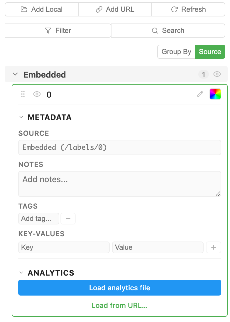
Every label renders as a row with the essentials on a single line:

• toggle visibility
• Color swatch: click to open the style popover
• Label name: double-click to rename
• Filter count badge: appears when analytics is loaded, showing how many filters are active
• EXT badge: only on external labels

Click the row to expand its detail panel below. There you'll find Metadata (Source / Notes / Tags / Key-values), plus the Analytics section if analytics is loaded.

Style: solid, random, or per-object

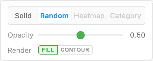
Click the color swatch on a label row to open the style popover. It holds the display controls for that label:

Control	Effect
Solid	Every object in the label shares a single colour (the one you pick below). Default for newly loaded labels.
Random	Each object gets a colour hashed from its ID. Different objects look different; the same object gets the same colour across reloads. Useful for visually distinguishing neighbouring cells without a segmentation-quality judgement.
Heatmap	Colour by a numeric column. Requires an analytics CSV. See the Analytics guide.
Category	Colour by a string column. Requires an analytics CSV.
Opacity slider	Blends the label layer with the image underneath. 0 hides the label; 1 makes it fully opaque.
FILL / CONTOUR	Two independent toggles for polygon labels. Fill paints the interior; contour draws a 1-px outline. Turn fill off for "outlines-only" view. Useful when you want to see the image through your segmentation.
Presets grid	16 curated colours: RGB primaries on top, muted variants on the bottom row. One click applies.
Hex / RGB inputs	Type #FF00AA or type the three RGB values directly. Synced bidirectionally.
More colors…	Opens the OS-native picker for any colour + eyedropper (Chrome / Edge).

Grouping

The Labels list groups by Source by default. Embedded labels sit under "Embedded", and each external label gets its own group header. You can switch to Group By key-value using the toolbar:

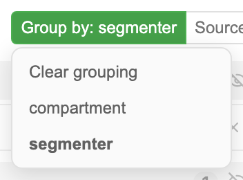
A key-value describes the whole mask, not the objects inside it, so useful keys are properties of the segmentation run: segmenter: stardist, model: nuclei_v2, version: 2026-03-11. Tag a dozen masks with segmenter and the list reorganises into a StarDist group and a Cellpose group, which is what you want when you are comparing runs on the same image.

Things that vary per object, like a cell's tissue class, do not belong here. Those live in an analytics table, one row per object. See Analytics & Phenotyping.

Drag the grip handle on the left of each group header to reorder groups. The group order also controls rendering z-order on the canvas. Later groups draw on top.

Worked example: multiple compartments

Segmentation usually gives you more than one mask. A typical run writes a set of compartments for the same objects, and they nest: nuclei sit inside cells, and cytoplasm is what is left when you subtract one from the other. Give each compartment its own colour and render mode and you can read all of them at once, in one view.

Here is a real setup on one well of a BBBC013 plate. A single segmentation run produced three masks, so all three arrive together under one source group.

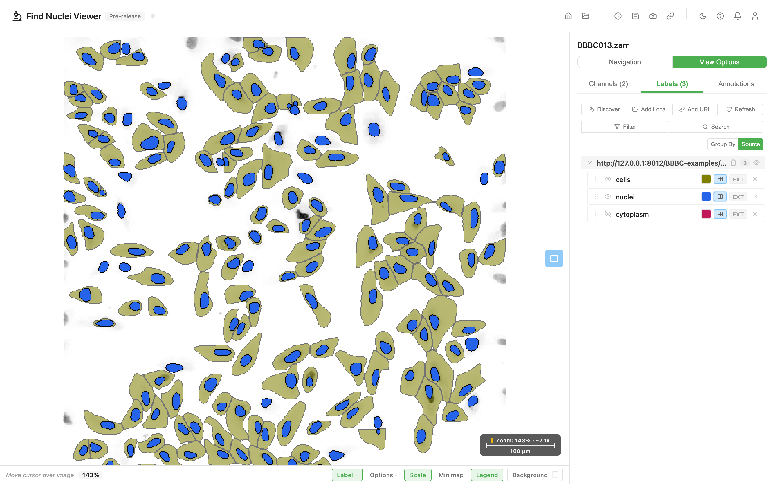
Position in list	Label	Colour	Render	Job it does
1 (drawn first, underneath)	cells	Solid olive, opacity 0.55	Fill + contour	Gives every object a body, so cell shape and packing read at a glance.
2 (drawn last, on top)	nuclei	Solid blue, opacity 1	Fill + contour	Sits inside the bodies, so you can see the nucleus each cell belongs to.
3	cytoplasm	Solid pink	Hidden	Styled, then switched off. One click brings it back when something needs checking.

Order decides what you see on top. Later in the list draws on top, so dragging cells above nuclei puts the bodies down first and lands the nuclei on them. Drag the two rows the other way and the bodies come forward instead. Whichever compartment you want to read is the one to keep at the bottom of the list.

Contour separates neighbouring objects. Turn CONTOUR on alongside FILL and every object gets its own edge, so two touching cells stay distinct while keeping the same colour. Keeping contour and switching fill off goes further: outlines give you shape and position while leaving the pixels underneath fully visible.

Opacity lets the layers underneath show through. The body layer runs at reduced opacity so the image reads through it, and the layer on top stays fully opaque so its colour comes through true. Opacity does its best work on the layers you are looking past.

The whole arrangement persists. Reload the image and the order, the per-layer colours, the render modes, the opacity and the hidden layer all come back.

Colouring by measurement

The colours above are one per mask. To give each object its own colour, from its area, its intensity, or a classification, load a measurement table and colour by a column. See Color by column for heatmaps and categories, and Phenotypes for named groups.

HCS Analytics in the Browser: 18,648 Nuclei, Zero Uploads picks up from exactly this point. It takes the same three masks on the same BBBC013 screen and carries them through to named phenotypes across the whole plate.

Search and filter

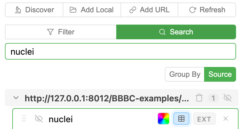
The toolbar row has a Filter dropdown and a Search input:

• Filter: show All / only Visible / only Hidden labels.
• Search: type part of a label name, tag, or metadata value. The list narrows to matches live.

Metadata: Source, Notes, Tags, Key-values

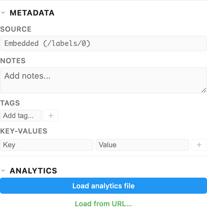
Expand a label's row and open the METADATA section. Four fields live here:

• Source: read-only, shows where the label came from (embedded path, local folder, URL).
• Notes: free-form text. "Run 2 from Cellpose, threshold 0.65."
• Tags: short chips you can add / remove. "validated", "needs-review".
• Key-values: structured key: value rows describing the mask as a whole. segmenter: cellpose, model: cyto3, version: 2026-03-11. Add one, then switch to Group By on the toolbar and the list reorganises by that key.

Metadata persists to IndexedDB per-label and survives reloads.

HCS plates

When you open a high-content-screening plate, labels work the same way but apply at the plate level. A label named nuclei is discovered on every populated well and renders consistently across all fields. See the HCS Plates guide for plate-specific controls (well navigation, field grid, plate overview).

Persistence

Everything you do in the Labels tab persists to your browser's IndexedDB, keyed by the image's URL or local folder handle:

• Visibility, colour mode, opacity, fill/contour state
• Label and group order, which is also the canvas z-order
• Notes, tags, key-values
• Which labels you've added external / URL-based
• Current group-by mode

Reload the page, reopen the image. Your label configuration is still there. The URL query string captures viewport state (zoom, center, active channels) but not label configuration; that lives in the browser locally.

Mobile

On phone viewports the Labels tab shows the row list and basic visibility toggles, but heatmap / category / phenotype coloring tabs are disabled. Per-object coloring needs an analytics CSV, and the File System Access API required to pick one doesn't exist on phones. Tablets show the full desktop UI.

Image credits

The screenshots on this page use a public whole-slide H&E section, a high-content screen and a fluorescence image from IDR. See Sample Data and Credits.

Next steps

• Want to colour cells by area, intensity, or any measurement? Analytics & Phenotyping.
• Drawing your own regions (not from a segmentation mask)? Annotations.
• Sharing your view with a reviewer? Sharing Views.
• Hosting your own label data? Data Server.