HCS Plates
Find Nuclei Viewer supports High-Content Screening (HCS) plate data in OME-ZARR format. Any plate format works: 96, 384, 1536-well, and custom layouts.
Once the plate is open, the question is usually which cells responded. HCS Analytics in the Browser: 18,648 Nuclei, Zero Uploads takes a segmented BBBC013 screen and answers that without leaving the image, which is the part a scatter plot cannot do.
Opening a plate
Open an HCS plate the same way as any other OME-ZARR dataset. Drag and drop, or paste a URL. The viewer detects the plate metadata and switches the sidebar to plate navigation.
View modes
A plate is three things at once: a single field, a well, and the whole layout. The Field / Well / Plate toggle at the top of the Navigation tab moves between them, and the rest of the panel follows whichever one is active.
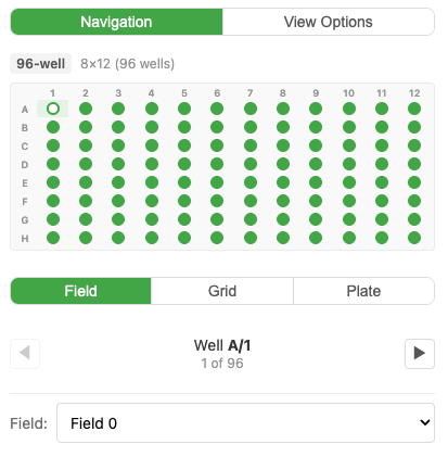
Field shows one field, exactly like any single image. Zoom, pan, and adjust channels as usual. This is where a plate opens, on the first field of the first populated well.
Well lays out every field of the current well side by side, so you can judge the whole well at once. It becomes available as soon as a well holds more than one field. On the 384-well plate above each well has a single field, which is why Well is greyed out there.
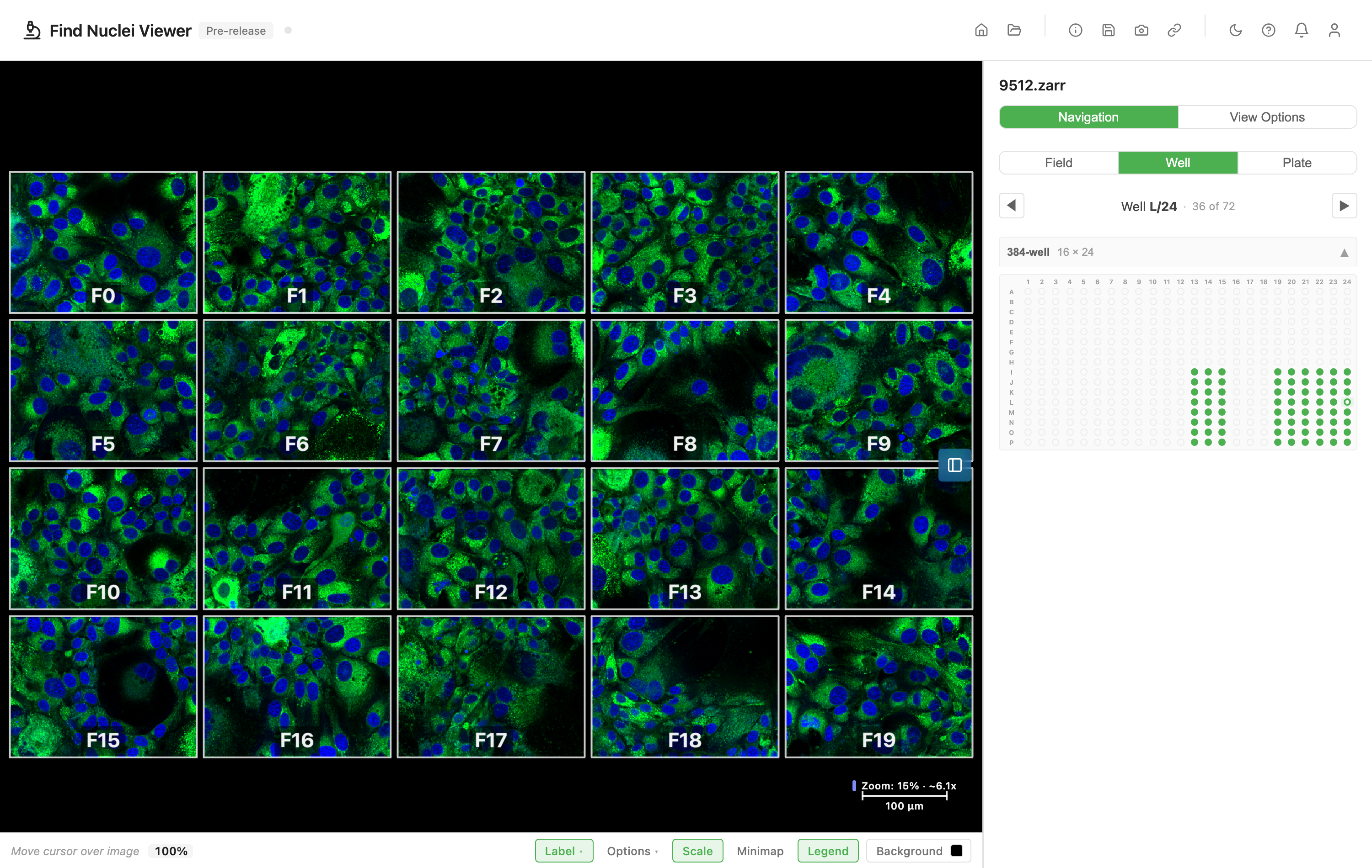
Plate renders every populated well in the plate layout, giving you the whole screen in one view. From here you can zoom smoothly all the way back down to individual cells: the viewer loads the right resolution across wells and fields as you go, so the plate overview and a single nucleus are the same continuous view.
Moving between wells
The navigator under the toggle steps through populated wells with the arrows, and tells you where you are: Well L/24 · 36 of 72. It counts populated wells only, so there are no empty stops to click past.
Below it, the plate grid draws the full layout with populated wells picked out. Click any well to jump straight to it. It collapses with the arrow on its header when you want the room.
When a well holds several fields, a field dropdown appears next to the well name. What it does depends on the mode:
- In Field view it picks which field you are looking at.
- In Plate view it picks which field index represents every well in the overview, so you can compare the same field position across the whole plate.
Labelling the tiles
In Well and Plate view, the Label control in the status bar chooses the text drawn on each tile: field ID (F0, F1, F2), well ID (A1, B3, G11), or none. If the plate carries well annotations, those appear as options too, so the grid can be labelled by dose, compound, or any other column your plate metadata provides.
Channels across the plate
Channel settings apply to every well and field at once. Pick a colour or set a contrast window in Field view and the whole plate follows, which is what makes a Plate view comparable across wells. All the controls work the same as anywhere else, so see the Channels guide for what each one does.
Labels and analytics
Segmentation masks work on plates, discovered across wells and rendered consistently on every field. Because scanning a plate for masks is a per-well operation, plates ask before they scan rather than doing it on open. The Labels guide covers that, and Analytics & Phenotyping covers colouring objects by measurement, which is where a plate becomes a plot.
Live Examples
| Example | Description |
|---|---|
| HCS Plate (v0.5, 5ch) | Multi-well plate, 5 channels, v0.5 |
| HCS Plate (v0.4, 2ch) | Multi-well plate, 20 fields per well, v0.4 |
Image credits
The screenshots on this page use plates from public collections. See Sample Data and Credits.